Reticulating Tibbles

python

deep learning

time series

Chunks of R and slithers of Python; in the caldron boil and bake

Author

Carl Goodwin

Published

May 1, 2024

Modified

May 1, 2024

What to do when a model is available (or installable) only in Python, but you code in R?

I want to try the deep-learning time-series package GluonTS on average house prices by London borough. There is an R wrapper for this, but also (at the time of writing) an open issue installing it on Apple silicon.

So, into the caldron boil and bake; a blended approach we will take.

Libraries (R)

library(conflicted)
library(tidyverse)
conflict_prefer_all("dplyr", quiet = TRUE)
library(paletteer)
library(scales)
library(janitor)
library(trelliscope)
library(reticulate)
library(clock)
library(glue)
library(gt)
library(tictoc)
library(patchwork)
library(rvest)
library(usedthese)

conflict_scout()

Theme (R)

theme_set(theme_bw())

n <- 5
palette <- "vangogh::Rest"

cols <- paletteer_d(palette, n = n)

tibble(x = 1:n, y = 1) |>
  ggplot(aes(x, y, fill = cols)) +
  geom_col(colour = "white") +
  geom_label(aes(label = cols |> str_remove("FF$")), 
             size = 4, vjust = 2, fill = "white") +
  annotate(
    "label",
    x = (n + 1) / 2, y = 0.5,
    label = palette,
    fill = "white",
    alpha = 0.8,
    size = 6
  ) +
  scale_fill_manual(values = as.character(cols)) +
  theme_void() +
  theme(legend.position = "none")

Read & Combine (R)

raw_df <- readRDS("raw_df") # file in github repo

# covid cases
covid_df <- tribble(
  ~date, ~covid_cases,
  "2026-12-31", 0, # optimistic assumption!
  "2025-12-31", NA,
  "2024-12-31", NA,
  "2023-12-31", 570463,
  "2022-12-31", 8665437,
  "2021-12-31", 9461237,
  "2020-12-31", 2327686
) |> 
  mutate(
    date = ymd(date), 
    covid_cases = zoo::na.approx(covid_cases)
    )

# mortgage rates
morgage_df <- str_c(
  "https://www.bankofengland.co.uk/boeapps/database/",
  "fromshowcolumns.asp?Travel=NIxAZxSUx&FromSeries=1&ToSeries=50&",
  "DAT=ALL&",
  "FNY=Y&CSVF=TT&html.x=66&html.y=26&SeriesCodes=", "IUMBV42",
  "&UsingCodes=Y&Filter=N&title=Quoted%20Rates&VPD=Y"
) |>
  read_html() |>
  html_element("#stats-table") |>
  html_table() |>
  clean_names() |>
  mutate(date = dmy(date)) |>
  filter(month(date) == 12) |> 
  rename(morg_rate = 2) |> 
  mutate(morg_rate = morg_rate / 100) |> 
  add_row(date = ymd("2024-12-31"), morg_rate = 0.0371) |> 
  add_row(date = ymd("2025-12-31"), morg_rate = 0.0320) |> 
  add_row(date = ymd("2026-12-31"), morg_rate = 0.0304) # poundf.co.uk/mortgage-rates

long_df <- raw_df |> 
  row_to_names(row_number = 1) |> 
  clean_names() |> 
  rename(district = na) |> 
  select(
    district, 
    date = ncol(raw_df),
    price = overall_average,
    volume = total_sales
    ) |> 
  filter(
    district != "Total", 
    !is.na(district), 
    .by = district
    ) |> 
  mutate(
    across(c(price, volume), as.numeric),
    date = date_build(date, 12, 31),
    district = factor(district)
    ) |> 
  full_join(covid_df, join_by(date)) |> 
  full_join(morgage_df, join_by(date)) |> 
  complete(district, date) |> 
  arrange(date, district) |> 
  group_by(date) |> 
  fill(covid_cases, morg_rate, .direction = "up") |> 
  ungroup() |> 
  drop_na(district) |> 
  arrange(district, date)

long_df |> glimpse()

Rows: 1,056
Columns: 6
$ district    <fct> BARKING AND DAGENHAM, BARKING AND DAGENHAM, BARKING AND DA…
$ date        <date> 1995-12-31, 1996-12-31, 1997-12-31, 1998-12-31, 1999-12-3…
$ price       <dbl> 50568, 51692, 56234, 63893, 69511, 84149, 94483, 118906, 1…
$ volume      <dbl> 1504, 1906, 2449, 2515, 2698, 2829, 3230, 3473, 3513, 3498…
$ covid_cases <dbl> NA, NA, NA, NA, NA, NA, NA, NA, NA, NA, NA, NA, NA, NA, NA…
$ morg_rate   <dbl> 0.0813, 0.0827, 0.0740, 0.0636, 0.0692, 0.0620, 0.0565, 0.…

long_df |> count(district) |> head()

district	n
BARKING AND DAGENHAM	32
BARNET	32
BEXLEY	32
BRENT	32
BROMLEY	32
CAMDEN	32

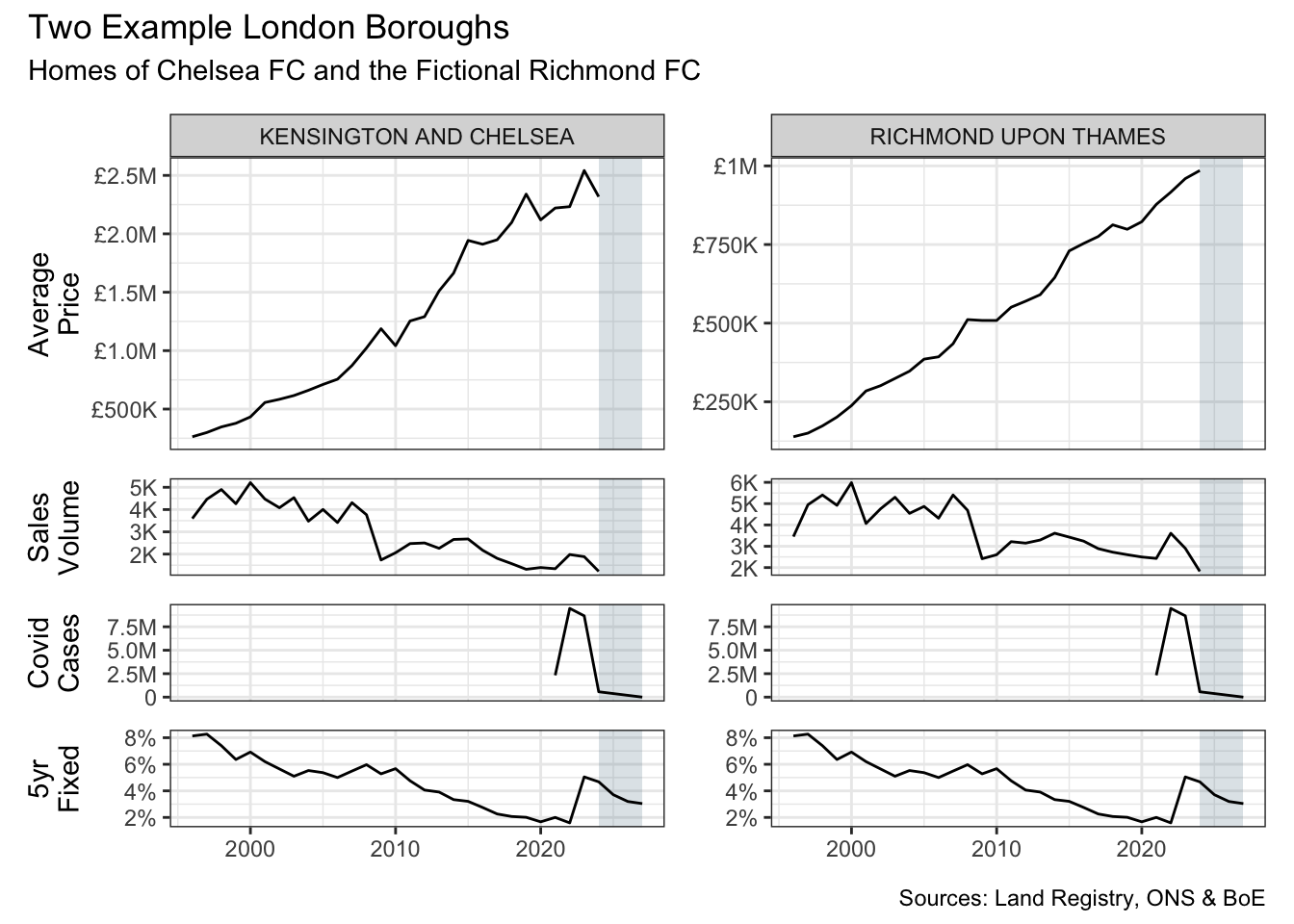
Visualise Examples (R)

long_df |>
  mutate(district = as.character(district)) |>
  filter(district %in% c("KENSINGTON AND CHELSEA", "RICHMOND UPON THAMES")) |>
  pivot_longer(-c(date, district), names_to = "var") |>
  mutate(var = fct_inorder(var)) |>
  split(~ district + var) |>
  imap(
    \(x, y) {
      scale_y <- if (str_ends(y, "price")) {
        scale_y_continuous(
          name = "Average\nPrice",
          label = label_currency(scale_cut = cut_short_scale(), prefix = "£")
        )
      } else if (str_ends(y, "volume")) {
        scale_y_continuous(
          name = "Sales\nVolume",
          labels = label_number(scale_cut = cut_short_scale())
          )
      } else if (str_ends(y, "covid_cases")) {
        scale_y_continuous(
          name = "Covid\nCases",
          labels = label_number(scale_cut = cut_short_scale())
          )
      } else {
        scale_y_continuous(
          name = "5yr\nFixed",
          labels = label_percent()
          )
      }
      remove_strip <- if (!str_ends(y, "price$")) theme(strip.text = element_blank())

      x |>
        ggplot(aes(date, value)) +
        annotate("rect",
          xmin = ymd("2023-12-31"), xmax = ymd("2026-12-31"),
          ymin = -Inf, ymax = Inf, alpha = 0.2, fill = cols[1]
        ) +
        geom_line() +
        scale_y +
        facet_wrap(~district, scales = "free_y") +
        remove_strip +
        labs(x = NULL)
    }
  ) |>
  wrap_plots(
    ncol = 2
  ) + plot_layout(
    heights = c(3, 1, 1, 1),
    axes = "collect_x",
    axis_titles = "collect"
  ) +
  plot_annotation(
    title = "Two Example London Boroughs",
    subtitle = "Homes of Chelsea FC and the Fictional Richmond FC",
    caption = "Sources: Land Registry, ONS & BoE"
  )

Install gluonTS (R)

py_install("gluonts", "r-reticulate", pip = TRUE, ignore_installed = TRUE)

py_list_packages("r-reticulate")

Model (Python)

By prefixing long_df with r., Python can access the R object.

import pandas as pd
import numpy as np
import json
import torch

from gluonts.dataset.pandas import PandasDataset
from gluonts.torch import DeepAREstimator
from gluonts.dataset.split import split
from gluonts.evaluation import make_evaluation_predictions, Evaluator
from itertools import tee
from lightning.pytorch.callbacks import EarlyStopping
from lightning.pytorch.loggers import CSVLogger
from lightning.pytorch import seed_everything

full_ds = PandasDataset.from_long_dataframe(
  r.long_df,
  item_id = "district",
  freq = "Y",
  target = "price",
  feat_dynamic_real = ["covid_cases", "morg_rate"],
  past_feat_dynamic_real = ["volume"],
  future_length = 3,
  timestamp = "date")
  
test_ds, _ = split(full_ds, offset = -1)
val_ds, _ = split(full_ds, offset = -2)
train_ds, _ = split(full_ds, offset = -3)
  
seed_everything(20, workers = True)

np.random.seed(123)
torch.manual_seed(123)


early_stop_callback = EarlyStopping("val_loss", min_delta = 1e-4, patience = 5)
logger = CSVLogger(".")

estimator = DeepAREstimator(
  freq = "Y", 
  hidden_size = 100,
  prediction_length = 1, 
  num_layers = 2,
  lr = 0.01,
  batch_size = 128,
  num_batches_per_epoch = 100,
  trainer_kwargs = {
    "max_epochs": 50,
    "deterministic": True,
    "enable_progress_bar": False,
    "enable_model_summary": False,
    "logger": logger,
    "callbacks": [early_stop_callback]
    },
  nonnegative_pred_samples = True)
  
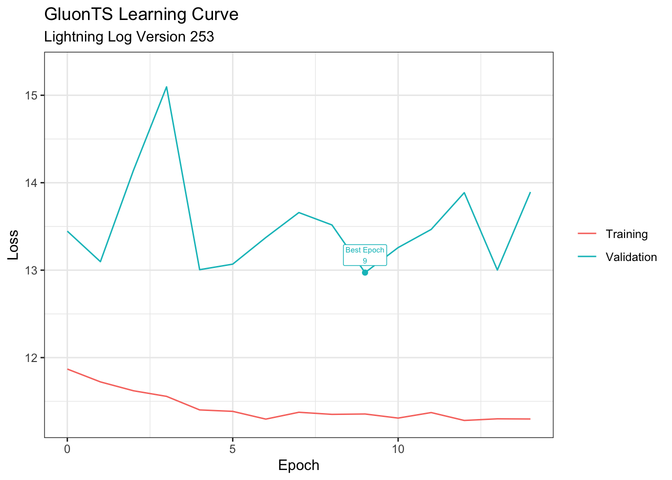
test_predictor = estimator.train(train_ds, val_ds)

Learning Curve (R)

version <- list.files("lightning_logs") |> parse_number() |> max()

log_df <- read_csv(str_c("lightning_logs/version_", version, "/metrics.csv"),
  show_col_types = FALSE
)

log_df |>
  select(-step) |>
  mutate(
    best_val = if_else(val_loss == min(val_loss, na.rm = TRUE), val_loss, NA),
    best_epoch = if_else(!is.na(best_val), glue("Best Epoch\n{epoch}"), NA)
  ) |>
  pivot_longer(ends_with("_loss"), values_drop_na = TRUE) |>
  mutate(name = case_match(
    name,
    "train_loss" ~ "Training",
    "val_loss" ~ "Validation",
  )) |>
  ggplot(aes(epoch, value, colour = name)) +
  geom_line() +
  geom_point(aes(y = best_val), show.legend = FALSE) +
  geom_label(
    aes(label = best_epoch),
    size = 2,
    nudge_y = 0.2,
    show.legend = FALSE
  ) +
  labs(
    title = "GluonTS Learning Curve",
    subtitle = glue("Lightning Log Version {version}"),
    x = "Epoch",
    y = "Loss",
    colour = NULL
  )

Test (Python)

test_fcast = list(test_predictor.predict(test_ds))

seed_everything(42, workers = True)

np.random.seed(123)
torch.manual_seed(123)

# Train and predict
forecast_it, ts_it = make_evaluation_predictions(
    dataset = train_ds, 
    predictor = test_predictor,
    num_samples = 1000
)

# Copy iterators
ts_it, targets = tee(ts_it) 
forecast_it, predictions = tee(forecast_it) 

# Calculate metrics
evaluator = Evaluator(quantiles=[0.05, 0.5, 0.95])
agg_metrics, item_metrics = evaluator(
    ts_it, 
    forecast_it, 
    num_series = len(test_ds)
)

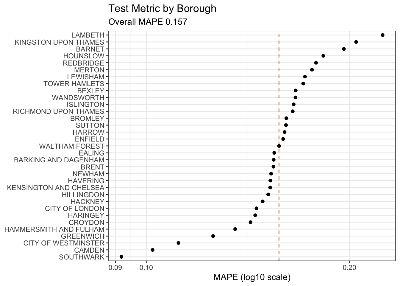
Metrics (R)

By prefixing agg_metrics with py$, R can access the Python object.

aggregated <- as.numeric(py$agg_metrics["MAPE"])

col <- compose(as.character, \(x) cols[x])

py$item_metrics |> 
  select(item_id, MAPE) |> 
  mutate(item_id = fct_reorder(item_id, MAPE)) |> 
  ggplot(aes(MAPE, item_id)) +
  geom_vline(xintercept = aggregated, linetype = "dashed", colour = col(2)) +
  geom_point() +
  scale_x_log10() +
  labs(
    title = "Test Metric by Borough", 
    subtitle = glue("Overall MAPE {round(aggregated, 3)}"), 
    x = "MAPE (log10 scale)", y = NULL
    )

Final Model (Python)

estimator = DeepAREstimator(
  freq = "Y", 
  hidden_size = 100,
  prediction_length = 3, 
  num_layers = 2,
  lr = 0.01,
  batch_size = 128,
  num_batches_per_epoch = 100,
  trainer_kwargs = {
    "max_epochs": 12,
    "deterministic": True,
    "enable_progress_bar": False,
    "enable_model_summary": False,
    },
  nonnegative_pred_samples = True)

seed_everything(42, workers = True)

np.random.seed(123)
torch.manual_seed(123)


final_predictor = estimator.train(full_ds)

future_fcast = list(final_predictor.predict(full_ds))

Forecast (R)

fc_ls = c(py$test_fcast, py$future_fcast)

years_df <- fc_ls |>
  map("mean_ts") |>
  map(as.data.frame.table) |>
  list_rbind() |>
  mutate(
    date = Var1,
    fcast = Freq,
    .keep = "unused"
  )

quantiles_df <- map(1:length(fc_ls), \(x) {
  fc_ls[[x]]$`_sorted_samples` |>
    as_tibble() |>
    reframe(
      across(everything(), \(x) quantile(x, probs = c(0.05, 0.1, 0.5, 0.9, 0.95))),
      quantile = c("pi90_low", "pi80_low", "median", "pi80_high", "pi90_high")
    ) |>
    pivot_longer(-quantile, names_to = "window") |>
    mutate(sample = x, district = fc_ls[[x]]$item_id)
}, .progress = TRUE) |>
  list_rbind() |>
  pivot_wider(names_from = quantile, values_from = value) |>
  bind_cols(years_df) |>
  pivot_longer(starts_with("pi"), names_to = c("pi", ".value"), names_pattern = "(.*)_(.*)") |>
  nest(.by = c(district, sample)) |>
  mutate(sample = row_number(), .by = district) |>
  unnest(data) |>
  mutate(pi_sample = str_c(`pi`, "-", sample) |> factor()) |>
  arrange(district, date, sample) |>
  mutate(date = str_c(date, "-12", "-31") |> ymd())

districts <- long_df |> summarise(n_distinct(district)) |> pull()

Trelliscope (R)

panels_df <- long_df |>
  left_join(quantiles_df, join_by(district, date)) |> 
  ggplot(aes(date, price)) +
  geom_line() +
  geom_ribbon(aes(y = median, ymin = low, ymax = high, fill = fct_rev(pi_sample)),
    alpha = 1, linewidth = 0) +
  geom_line(aes(date, median), colour = "white") +
  scale_fill_manual(values = col(c(1, 1, 5, 5))) +
  scale_y_continuous(labels = label_currency(scale_cut = cut_short_scale(), prefix = "£")) +
  facet_panels(vars(district), scales = "free_y") +
  labs(
    title = glue("Price Forecasts for {districts} Postal Districts"), 
    subtitle = "Backtest & Future Forecasts with 80 & 90% Prediction Intervals",
    caption = "DeepAR: Probabilistic Forecasting with Autoregressive Recurrent Networks",
    x = NULL, y = "Avg Price", fill = "Prediction\nInterval"
    ) +
  theme(legend.position = "none")

slope <- \(x, y) coef(lm(y ~ x))[2]

summary_df <- long_df |> 
  summarise(
    last_price = nth(price, -4), 
    slope = slope(date, price),
    .by = district)

panels_df |>
  as_panels_df(as_plotly = TRUE) |>
  as_trelliscope_df(
    name = "Average London House Prices",
    description = str_c(
      "Time series of house prices by London post code district ",
      "sourced from HM Land Registry Open Data."
    )
  ) |>
  left_join(summary_df, join_by(district)) |>
  set_default_labels(c("district", "last_price")) |>
  set_var_labels(
    district = "Post Code District",
    last_price = "Last Year's Avg Price"
  ) |>
  set_default_sort(c("last_price"), dirs = "desc") |>
  set_tags(
    stats = c("last_price", "slope"),
    info = "district"
  ) |>
  set_theme(
    primary = col(1),
    dark = col(1),
    light = col(5),
    light_text_on_dark = TRUE,
    dark_text = col(1),
    light_text = col(5),
    header_background = col(1),
    header_text = NULL
  ) |>
  view_trelliscope()

R Toolbox

Summarising below the packages and functions used in this post enables me to separately create a toolbox visualisation summarising the usage of packages and functions across all posts.

used_here()

Package	Function
base	as.character[2], as.numeric[1], c[14], col[8], factor[2], if[4], is.na[2], length[1], library[14], list[2], list.files[1], max[1], min[1], ncol[1], readRDS[1], round[1], saveRDS[1], split[4]
clock	date_build[1]
conflicted	conflict_prefer_all[1], conflict_scout[1]
dplyr	across[2], arrange[3], bind_cols[1], case_match[1], count[1], filter[3], full_join[2], group_by[1], if_else[2], join_by[4], left_join[2], mutate[15], n_distinct[1], nth[1], pull[1], reframe[1], rename[2], row_number[1], select[3], summarise[2], ungroup[1], vars[1]
forcats	fct_inorder[1], fct_reorder[1], fct_rev[1]
ggplot2	aes[10], annotate[2], element_blank[1], facet_wrap[1], geom_col[1], geom_label[2], geom_line[4], geom_point[2], geom_ribbon[1], geom_vline[1], ggplot[5], labs[4], scale_fill_manual[2], scale_x_log10[1], scale_y_continuous[5], theme[3], theme_bw[1], theme_set[1], theme_void[1]
glue	glue[4]
janitor	clean_names[2], row_to_names[1]
lubridate	dmy[1], month[1], ymd[7]
paletteer	paletteer_d[1]
patchwork	plot_annotation[1], plot_layout[1], wrap_plots[1]
pillar	glimpse[1]
purrr	compose[1], imap[1], list_rbind[3], map[4]
readr	parse_number[1], read_csv[2]
reticulate	py_install[1], py_list_packages[1]
rvest	html_element[1], html_table[1]
scales	cut_short_scale[4], label_currency[2], label_number[2], label_percent[1]
stats	coef[1], lm[1], quantile[1]
stringr	str_c[7], str_ends[4], str_remove[1]
tibble	add_row[3], as_tibble[1], tibble[1], tribble[1]
tictoc	tic[1], toc[1]
tidyr	complete[1], drop_na[1], fill[1], nest[1], pivot_longer[4], pivot_wider[1], unnest[1]
tidyselect	ends_with[1], everything[1], starts_with[1]
trelliscope	as_panels_df[1], as_trelliscope_df[1], facet_panels[1], set_default_labels[1], set_default_sort[1], set_tags[1], set_theme[1], set_var_labels[1], view_trelliscope[1]
usedthese	used_here[1]
utils	head[1]
xml2	read_html[1]
zoo	na.approx[1]